2014 unit cells
Download files for version 2 beta
The downloaded archive contains Quokka3 settingsfiles for all of the input parameter sets presented in (Fell et al. 2015), namely a conventional, PERC, n-PASHA, HJT, ANU-IBC and UNSW-PERL cell. For each cell type a settingsfile exists where the the skins are defined by their lumped properties. For the PERC cell and additional settingsfile is included which defines a much more complete and detailed model of the same cell. It comprises:
- detailed emitter properties (dopant profile, surface SRH), thus using the multiscale approach,
- a ‘busbar-enhanced’ unit cell geometry,
- light trapping via the ‘local-lumped’ Z approach, accounting for the different internal reflection properties of the different rear-side skin regions.
Download files for version 2 beta
Conventional and PERC cells
2018 Trina PERC cell, multi-domain
Download files for version 2 beta
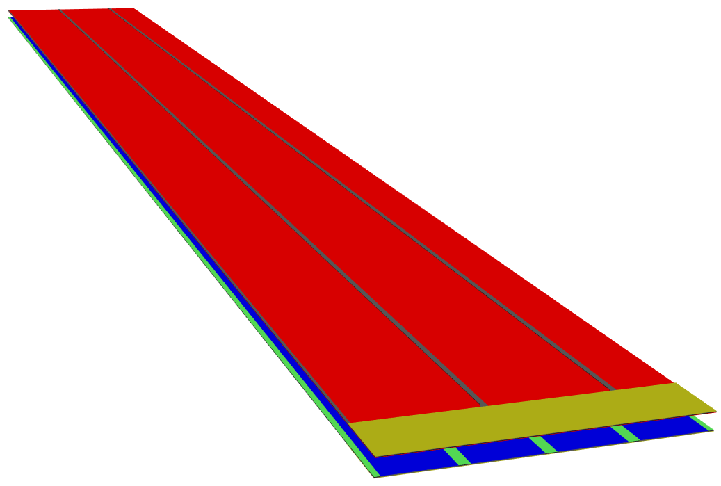
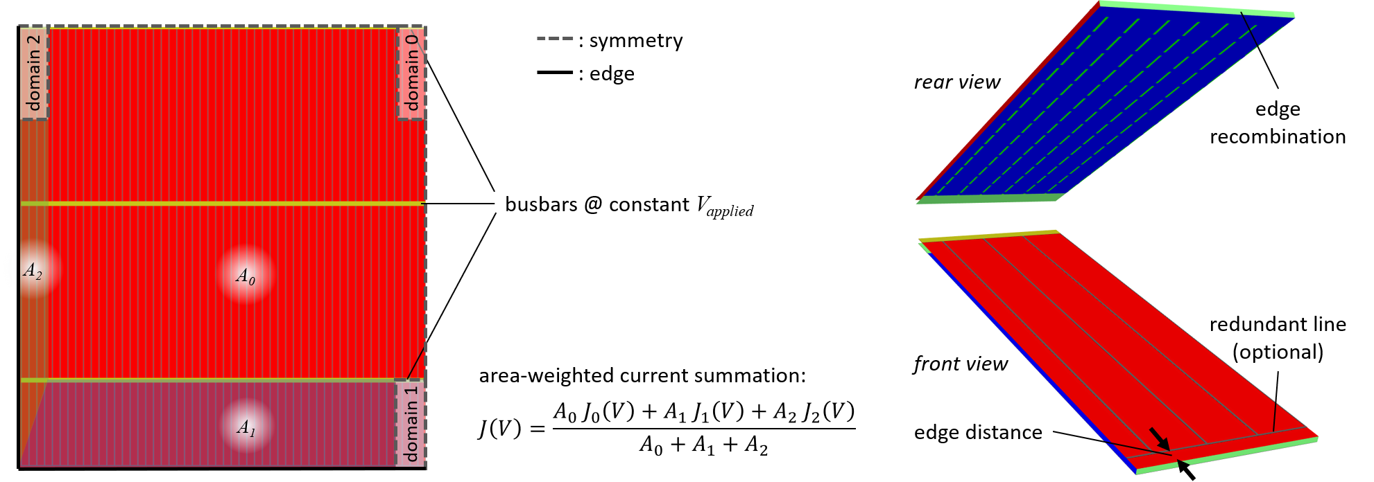
This examples defines a Trina PERC cell as manufactured during ramp-up of a production line. The input parameters were published in (A. Fell and Altermatt 2018b) and (A. Fell and Altermatt 2018a).
Three settingsfiles are included:
- a ‘busbar-enhanced’ unit cell type using the “front and rear contact unit cell” syntax for a 5 busbar layout as published
- a multidomain approach to model the full-size of the cell including edge effects
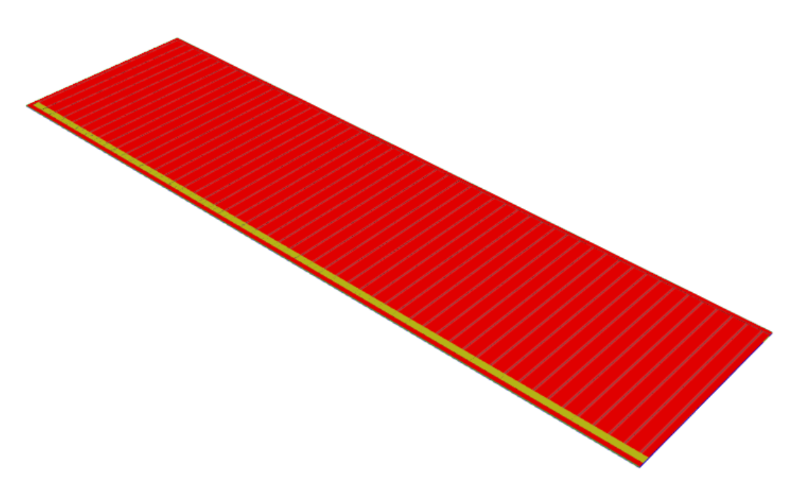
- additionally a multidomain approach for a shingle layout with otherwise identical properties (not representing a real cell)
Download files for version 2 beta
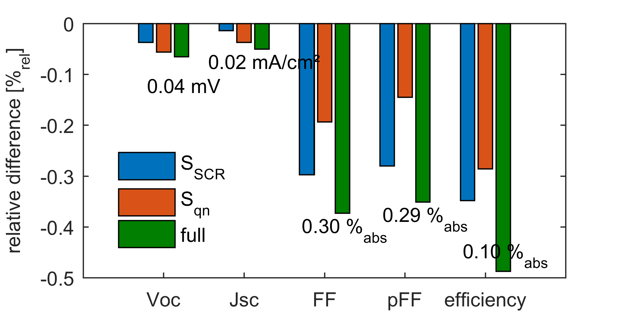
PERC: half-cell with edge recombination
This examples shows how to define a PERC half-cell having high recombination at the cut-edge. It is taken from (Andreas Fell, Sträter, et al. 2017), and more details on the edge recombination model can be found in (A. Fell, Schön, et al. 2018). It uses the ‘generic’ Syntax.
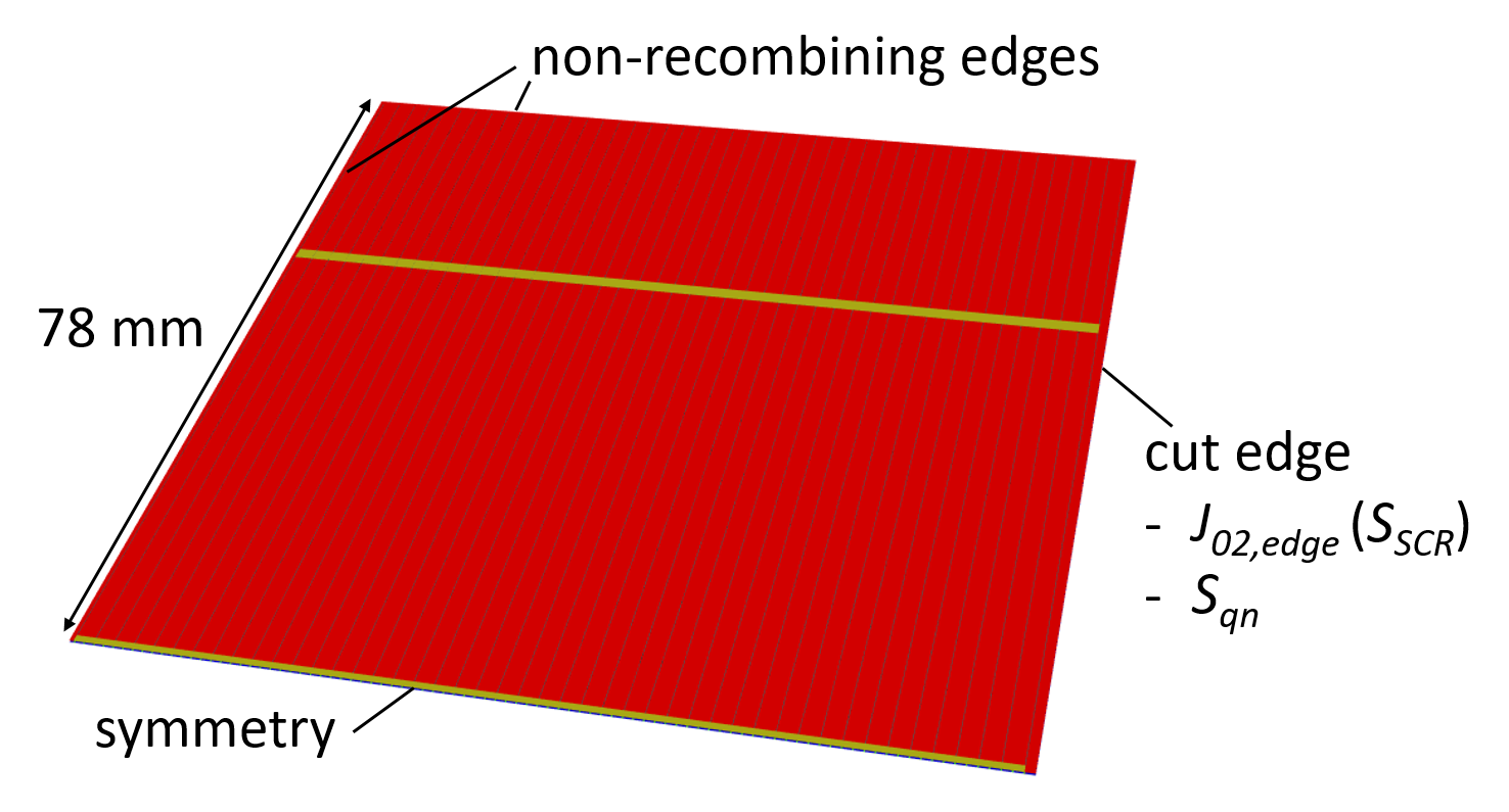
By switching the edge recombination on off, implemented by sweeping the respective settings, one can simply calculate the losses by comparing the two simulations. In the settingsfile a light JV curve solution-type is set, giving the light JV parameters. Additionally the solution-type can be changed to a suns-Voc curve to determine the pFF loss. With Quokka3 one can independently set the edge loss contributions from the SCR (via J02,edge) and at the quasi-neutral bulk edge, which is summarized in the below plot.
Conventional: bulk lifetime variation of mc cell
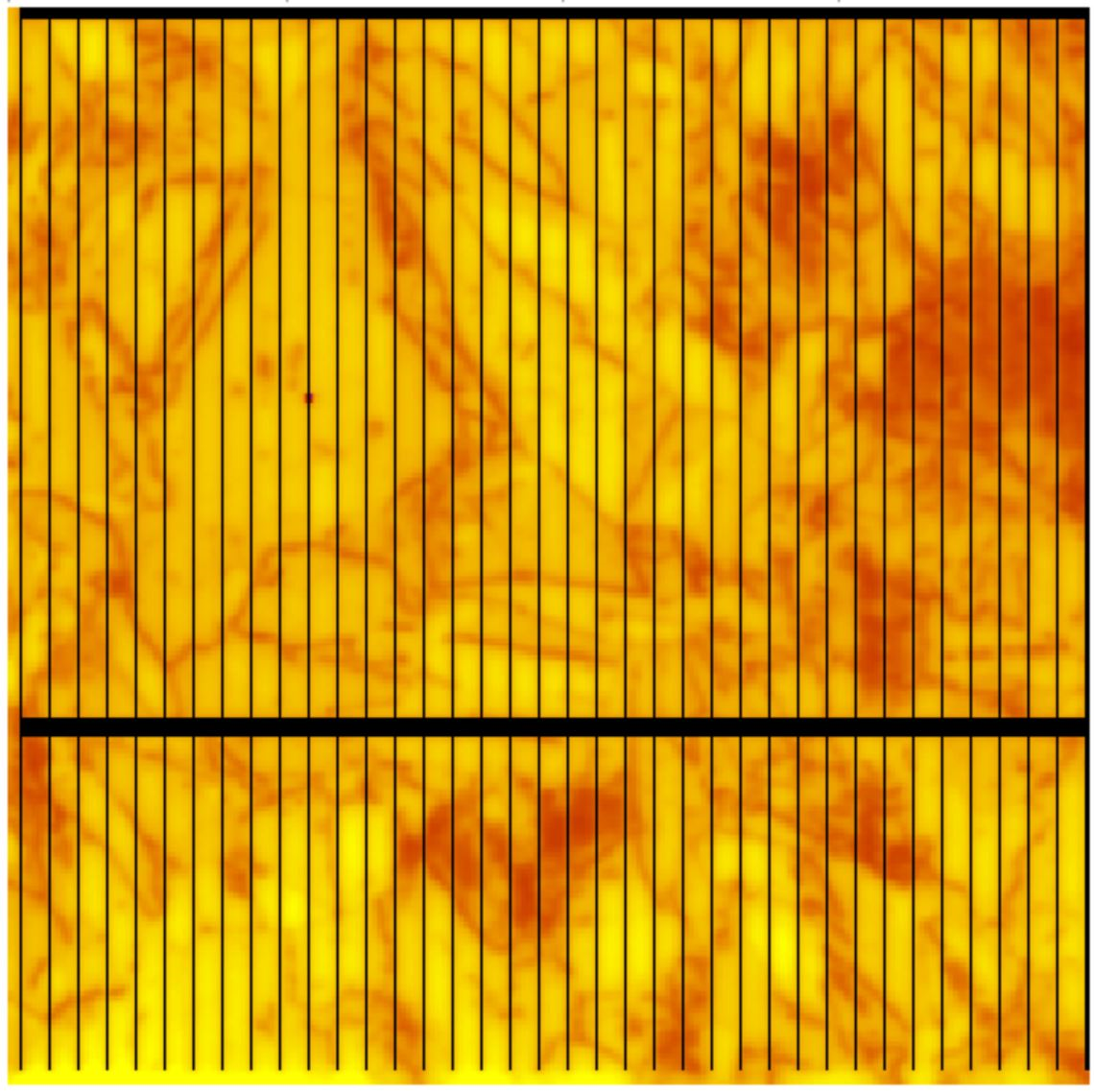
This example shows the capability of Quokka3 to define a spatially varying and injection-dependent bulk lifetime, from lifetime images taken at various injection levels. It uses the input parameters of the conventional full-area Al-BSF cell of (Fell et al. 2015), but replacing the bulk lifetime by lifetime images. The full cell geometry is conveniently created using the simplified ‘front and rear contact full cell’ syntax. The downloaded files also contain a Matlab and a Python script to convert a series of lifetime images into the required input file format for Quokka3.
A few things should be noted:
- As Quokka3 expects the actual bulk lifetime to be defined, one should provide images corrected for optical and electrical smearing effects.
- When using established de-smearing algorithms to correct for carrier diffusion, the resulting images may contain artefacts resulting in non-sensible lifetime values and / or a jumpy injection dependence at some pixels. This may lead to convergence errors in Quokka3, and therefore requires some user-effort into sanity checking and smoothing the input images (see the Matlab script for an exemplary approach).
- A ‘user’ mesh quality is required to be used, as one needs to prevent too large elements to keep a a desired spatial resolution of the results, but a ‘standard’ or ‘fine’ mesh quality is prohibitive for such large area simulations. See the settingsfile for a sensible mesh inputs.
- Such simulations are computationally expensive due to the required mesh sizes. The examples runs well over 1 hour.
Bifacial
Bifacial n-PERT cell
This example defines a bifacial n-PERT cell simulating true simultaneous front and rear illumination. The front and rear skins are defined in detail by dopant profiles etc.. The example can thus correctly reproduce front and rear quantum efficiency measurements, accounting for collection losses within both the front and rear diffusion.
It uses a ‘busbar-enhanced’ unit cell geometry, allowing for varying busbar number, front pitch, and rear pitch, fully considering the impact on metal grid resistance, contact recombination, and shading.
TOPCon
##Fraunhofer ISE record cell
This examples defines the Fraunhofer ISE 25.8% efficient TOPCon cell, as published in (Richter et al. 2017).
It is shown how to use Quokka3’s MIS functionality to describe passivating contact physics, in this case the non-ohmic resistivity of the tunneling contact, see (A. Fell, Feldmann, et al. 2018) and the modelling guide for details. The two different settingsfiles show how the MIS contact resistivity can be modelled either by a detailed skin approach or lumped skin approach. In the detailed skin (multiscale) approach the potential drop over the insulator as well as the interplay of band-bending and surface recombination is resolved. Those effects are not resolved in the lumped skin approach, where the effective recombination of the contact system is defined by a lumped \(J_{0,skin}\), which is numerically faster and more robust.
Skinsolver
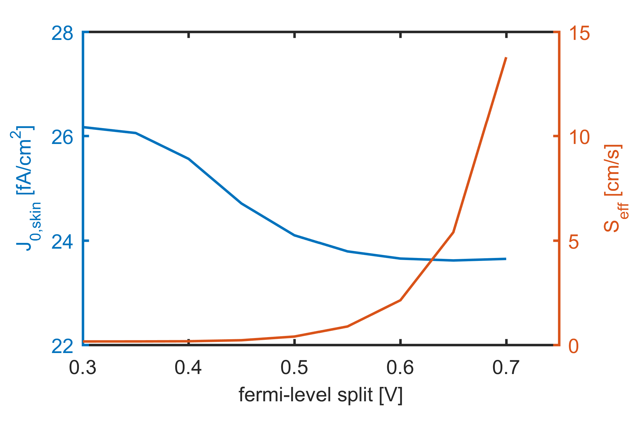
Al2O3 passivated silicon
This example shows how to use the skinsolver via the ‘near-surface skin’ syntax to model the effective properties of an Al3O3 passivated silicon surface with parameters taken from (Fell et al. 2015) (originally derived by (Black and McIntosh 2013)). The Al2O3 has a high surface charge, and moderate surface recombination velocities. By varying the bulk-side fermi-level split, the injection dependence of the effective recombination is revealed. It is shown that for the chosen surface charge, \(S_{eff}\) is strongly injection dependent, whereas \(J_{0,skin}\) can (only) approximately be considered a constant effective properties of the passivation. Further it can be observed that those properties are highly sensitive to the choice of material property models (e.g. BGN model), indicating a substantial unavoidable uncertainty in detailed modeling of silicon surfaces passivated by highly charged layers.
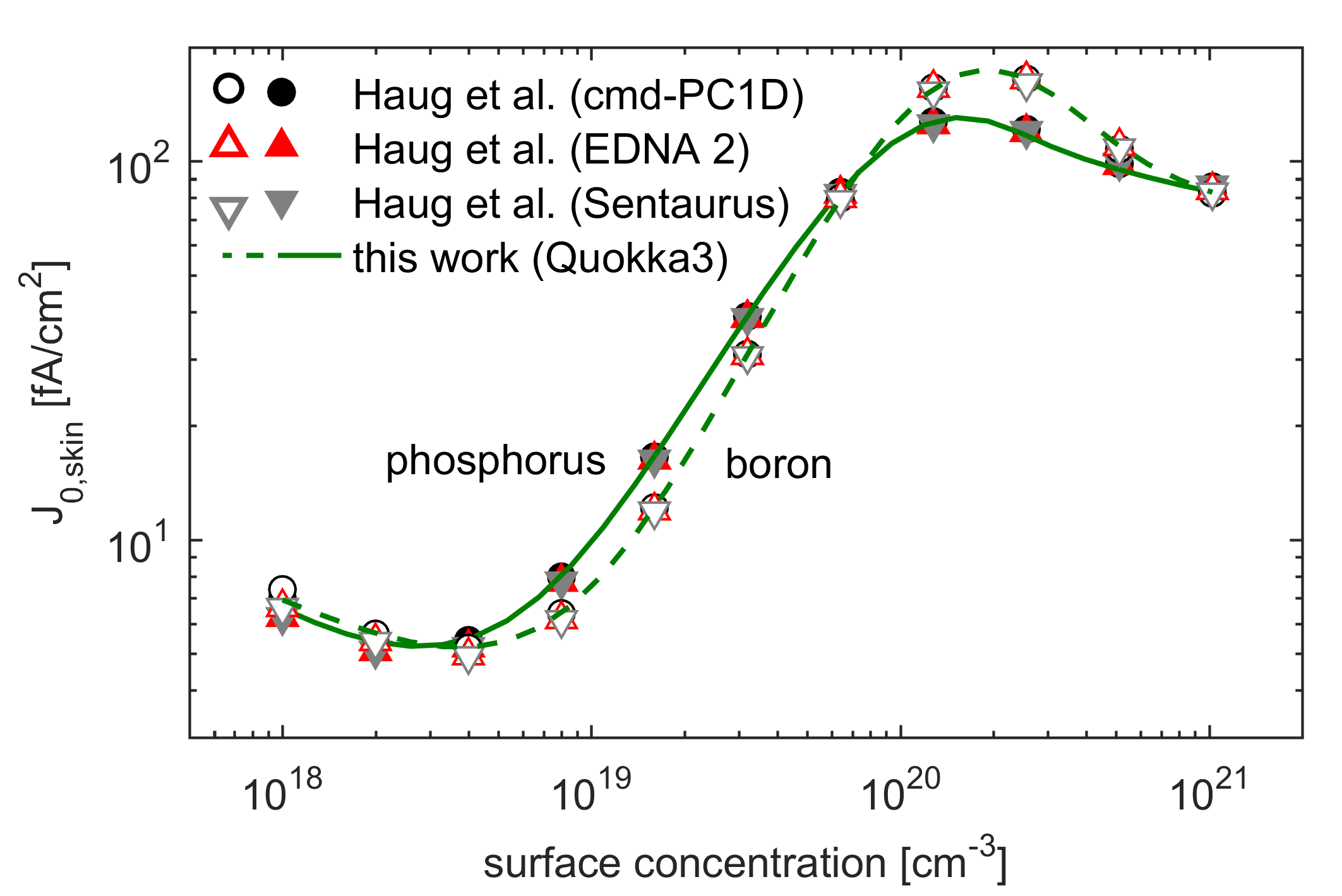
J0 of phosphorus and boron diffused silicon surfaces
This example simulates the \(J_{0,skin}\) for phosphorus and boron doping profiles with varying peak concentration. It replicates the data shown in Fig. 4 a) of (Andreas Fell, Schoen, et al. 2017), where it is compared against the equivalent simulations performed with cmd-PC1D, EDNA2 and Sentaurus presented in (Haug et al. 2014). It uses the skinsolver via the ‘near-surface skin’ syntax. The settingsfiles are prepared that it can be switched to simulate the skin’s QE-curve, by setting the appropriate solution type and enabling the illumination. The only output of a skin’s QE-curve is the collection efficiency CE, which for short-wavelengths equals the IQE of a cell with the respective skin at the front.
Ohmic
Cox and Strack MIS resistance structure
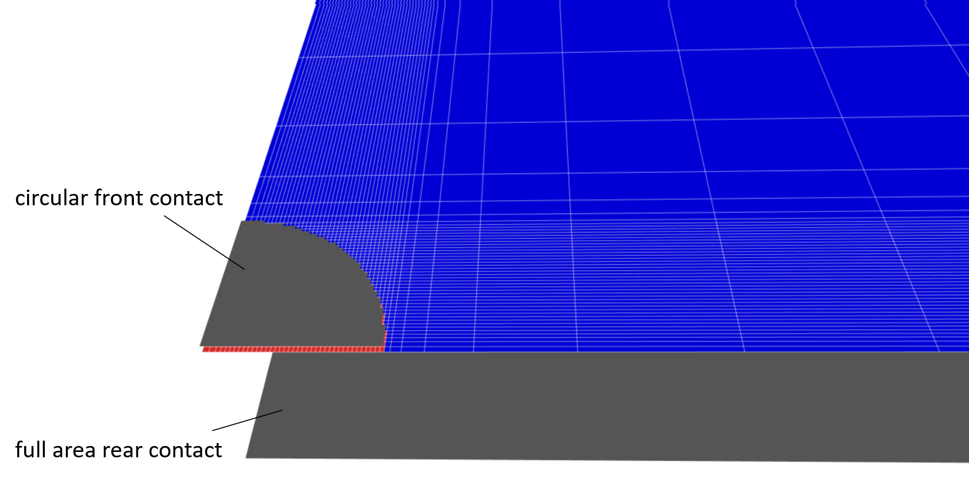
This example simulates the resistance of a Cox and Strack structure (Cox and Strack 1967), which besides the TLM method is popular in PV to determine the specific contact resistivity. The commonly applied analytical formulas to calculate the resistance of such a structure inhibit simplifying assumptions and approximations. These are for example an approximate formula for the bulk crowding resistance, the assumption of uniform current density through the contact, or neglecting finite perimeter effects. Numerical simulations can omit those assumptions and thereby result in a very accurate prediction of the total resistance. Further the simulation can be extended to account for e.g. a sheet resistance of the skin (e.g. a diffusion), or of the metal (by additionally defining pads to consider the position of measurement pins).
This is example features an MIS-type front contact, resulting in a non-ohmic JV-characteristic.
As Quokka3 uses a rectangular mesh, resolving the circular front contact does require at least a ‘standard’ mesh quality setting to sufficiently approximate to circular geometry.
In the settingsfile a sweep both of the circle diameter and the contact resistivity is defined. The resulting resistances can be used to compare to experimental data, and by matching them determine the experimental contact resistivity. Note that due to a quarter symmetry is being simulated, the simulated resistance needs to quartered to compare to measurements.
4PP resistance of CTLM structure
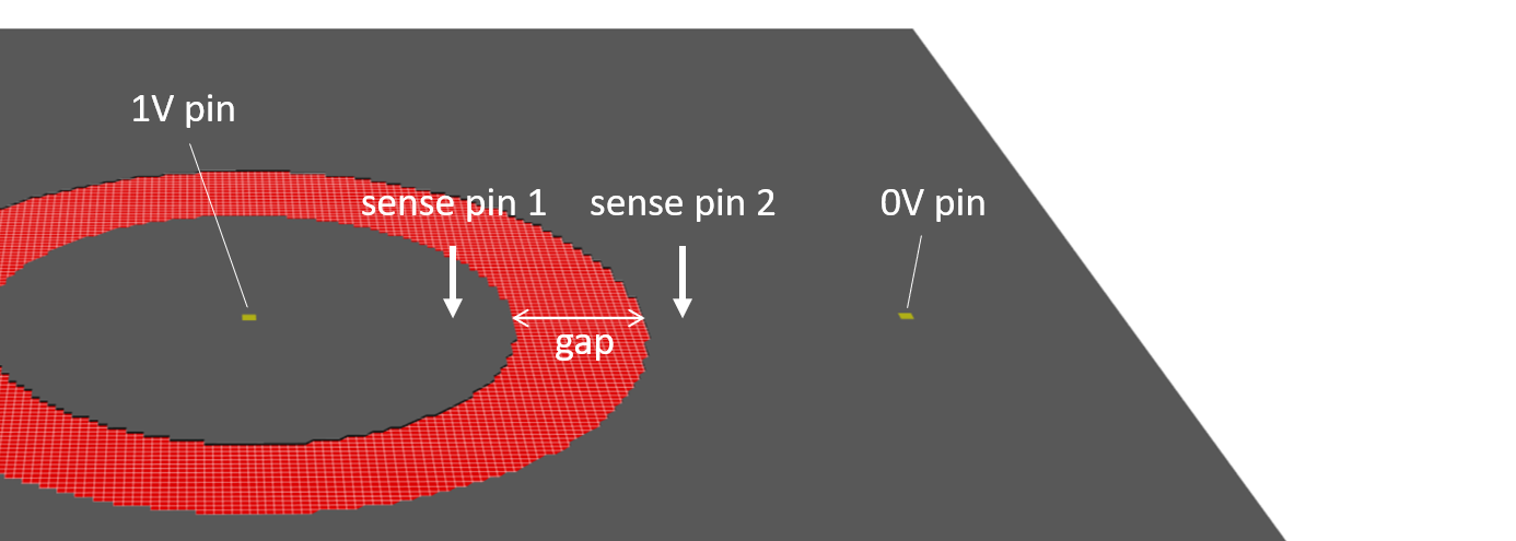
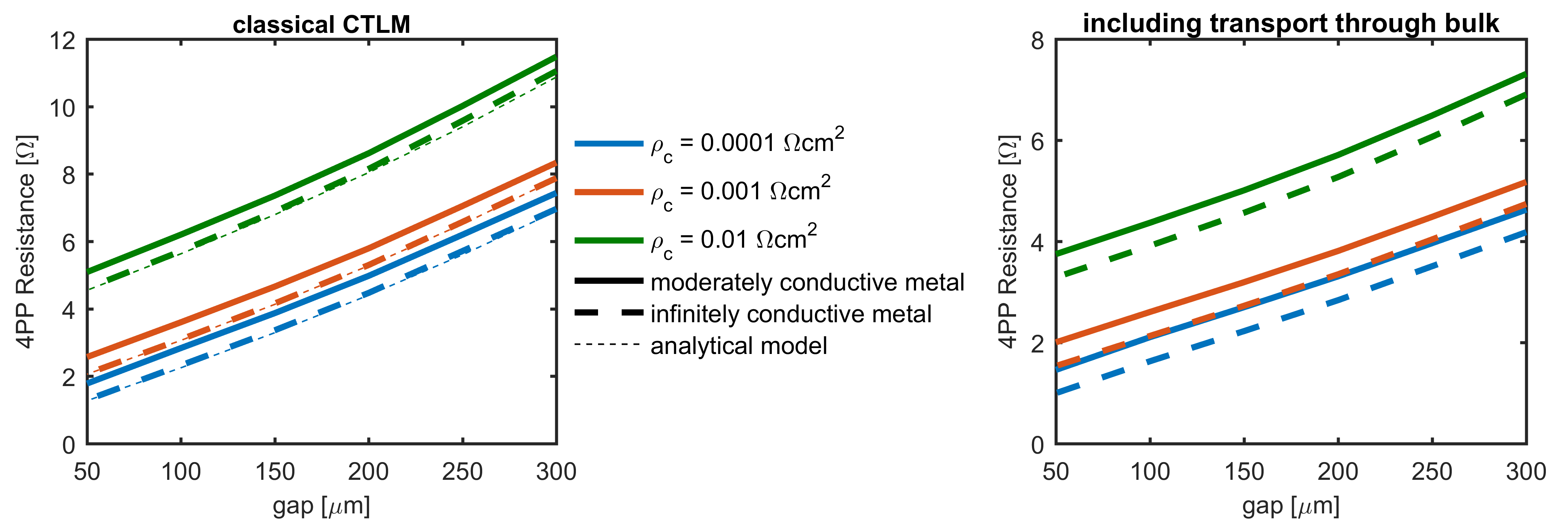
This example simulates the resistance of a CTLM structure. The settings define Probes along with small PadFeatures, representing the sense and current pins in a four-point-probe (4PP) setup, respectively. From the simulation result, the 4PP resistance can then calculated by the difference of the sensed voltage divided by the total current: \(R_{4PP}=\frac{V_{sense1}-V_{sense2}}{I_{term}}\).
For illustration, below the results for different scenarios are plotted: moderately vs. infinitely conducting metal features, with and without current transport through the bulk, in each case varying the contact resistivity and gap size. For the case of infinitely conductive metal and no current transport through the bulk, an analytical treatment is possible, which is in very good agreement with the simulation result.
#References
Black, Lachlan E., and Keith R. McIntosh. 2013. “Modeling Recombination at the Si–Al O Interface.” IEEE Journal of Photovoltaics 3 (3): 936–43.
Cox, RH, and H Strack. 1967. “Ohmic Contacts for Gaas Devices.” Solid-State Electronics 10 (12): 1213–8.
Fell, A., and P. P. Altermatt. 2018a. “A Detailed Full-Cell Model of a 2018 Commercial Perc Solar Cell in Quokka3.” IEEE Journal of Photovoltaics. https://doi.org/10.1109/JPHOTOV.2018.2863548.
———. 2018b. “Detailed 3D Full-Cell Modeling in Quokka3: Quantifying Edge and Solder-Pad Losses in an Industrial Perc Cell.” In Silicon Pv 2018. https://www.researchgate.net/profile/Andreas_Fell/publication/324115468_Detailed_3D_Full-Cell_Modeling_in_Quokka3_Quantifying_Edge_and_Solder-Pad_Losses_in_an_Industrial_PERC_Cell/links/5abea98ca6fdcccda65a0685/Detailed-3D-Full-Cell-Modeling-in-Quokka3-Quantifying-Edge-and-Solder-Pad-Losses-in-an-Industrial-PERC-Cell.pdf.
Fell, A., F. Feldmann, C. Messmer, M. Bivour, M. C. Schubert, and S. W. Glunz. 2018. “Adaption of Basic Metal–Insulator–Semiconductor (Mis) Theory for Passivating Contacts Within Numerical Solar Cell Modeling.” IEEE Journal of Photovoltaics. https://doi.org/10.1109/JPHOTOV.2018.2871953.
Fell, A., K. R. McIntosh, P. P. Altermatt, G. J. M. Janssen, R. Stangl, A. Ho-Baillie, H. Steinkemper, et al. 2015. “Input Parameters for the Simulation of Silicon Solar Cells in 2014.” IEEE Journal of Photovoltaics 5 (4): 1250–63. https://doi.org/10.1109/JPHOTOV.2015.2430016.
Fell, Andreas, Jonas Schoen, Martin C. Schubert, and Stefan W. Glunz. 2017. “The Concept of Skins for Silicon Solar Cell Modeling.” Solar Energy Materials and Solar Cells, 173 (Supplement C): 128–33. https://doi.org/10.1016/j.solmat.2017.05.012.
Fell, Andreas, Hendrik Sträter, Matthias Müller, Heiko Steinkemper, Jonas Schön, Martin Hermle, Martin C. Schubert, D. H. Neuhaus, and Stefan W. Glunz. 2017. “Modeling of Edge Recombination Losses in Half-Cells.” In 34th European Photovoltaic Solar Energy Conference and Exhibition. https://www.ise.fraunhofer.de/content/dam/ise/de/documents/publications/conference-paper/33-eupvsec-2017/Fell_2CV236.pdf.
Fell, A., J. Schön, M. Müller, N. Wöhrle, M. C. Schubert, and S. W. Glunz. 2018. “Modeling Edge Recombination in Silicon Solar Cells.” IEEE Journal of Photovoltaics PP (99): 1–7. https://doi.org/10.1109/JPHOTOV.2017.2787020.
Haug, Halvard, Achim Kimmerle, Johannes Greulich, Andreas Wolf, and Erik Stensrud Marstein. 2014. “Implementation of Fermi–Dirac Statistics and Advanced Models in Pc1d for Precise Simulations of Silicon Solar Cells.” Solar Energy Materials and Solar Cells 131 (0): 30–36. https://doi.org/10.1016/j.solmat.2014.06.021.
Richter, Armin, Jan Benick, Frank Feldmann, Andreas Fell, Martin Hermle, and Stefan W. Glunz. 2017. “N-Type Si Solar Cells with Passivating Electron Contact: Identifying Sources for Efficiency Limitations by Wafer Thickness and Resistivity Variation.” Solar Energy Materials and Solar Cells 173 (Supplement C): 96–105. https://doi.org/10.1016/j.solmat.2017.05.042.